🚦 Congestion Control
How senders share a finite network without collapsing it: congestion collapse and the AIMD feedback loop, slow start and congestion avoidance, loss-based recovery, CUBIC for high-BDP paths, BBR and delay-based control, and fairness, AQM, ECN and datacenter congestion.
8.1 Why congestion control exists
Congestion is a shared-resource failure. A packet network is built from links, switches, routers, NIC queues, DMA rings, software queues, and scheduler decisions. Every one of those places has finite service rate and finite buffering. If the senders feeding a bottleneck collectively inject packets faster than the bottleneck can transmit them, the excess waits in a queue or is dropped. For a short burst, buffering is useful. For sustained overload, buffering just delays the visible failure. The queue grows, RTT rises, and eventually packets are discarded.
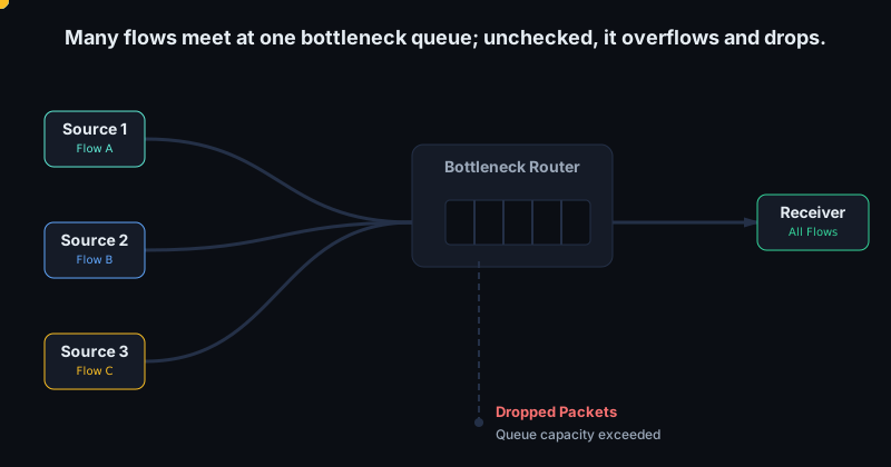
That sounds ordinary until retransmission enters the system. A reliable transport interprets missing data as work to do again. If many hosts keep transmitting new data while also retransmitting data that was already dropped, the network spends more of its finite capacity carrying packets that will not advance any application byte stream. Offered load rises, but useful throughput falls. This is congestion collapse: links are busy, interrupt paths are hot, queues are full, but delivered goodput drops because the control loop is wrong.
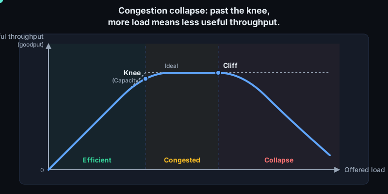
The early Internet hit this problem in practice. Van Jacobson and Michael Karels opened their 1988 SIGCOMM paper by describing the October 1986 Internet congestion collapses, where throughput between Lawrence Berkeley Laboratory and UC Berkeley fell dramatically despite the underlying links still existing. The lesson was not that TCP needed a bigger retransmission timer, or that routers needed infinite memory. The lesson was that end hosts had to stop treating the network as an invisible pipe. A sender must estimate how much data the path can absorb and must reduce its sending rate when the path shows signs of overload.
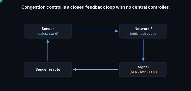
This is easy to say and hard to do because the Internet has no central scheduler for ordinary flows. A TCP sender usually does not know the bottleneck link rate, the number of competing flows, the queue depth in a router, whether the bottleneck is a WAN link, a top-of-rack uplink, a Wi-Fi hop, a policer, or a host receive path. It sees only indirect feedback: ACK timing, missing ACKs, duplicate ACKs, retransmission timeouts, sometimes ECN marks, and local signals such as pacing state and socket buffer pressure. Congestion control is the discipline of turning those weak signals into a stable distributed feedback loop.
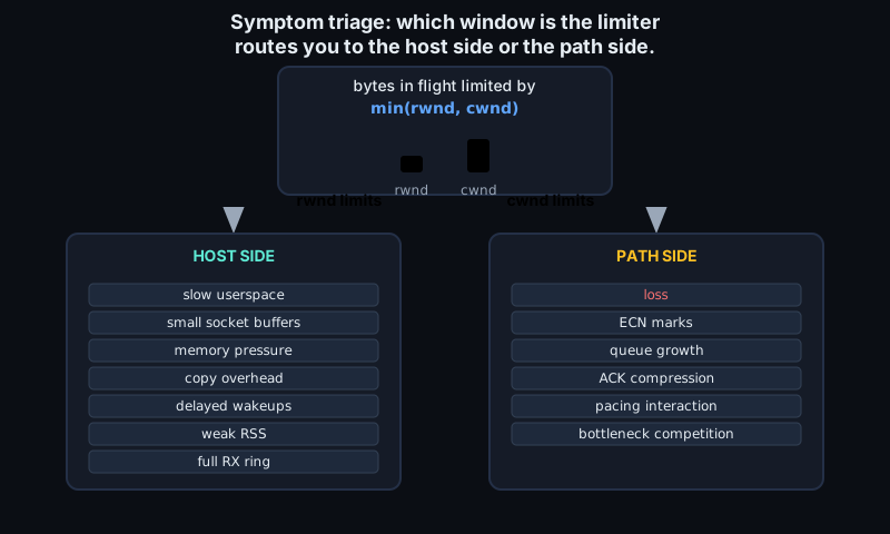
The first distinction to keep clean is flow control versus congestion control. Flow control protects the receiver. The receiver advertises rwnd, the receive window, saying how many more bytes it can accept without overflowing its socket buffer. If an application stops reading, rwnd shrinks, possibly to zero, even if the network is empty. Congestion control protects the network path. The sender maintains cwnd, the congestion window, its estimate of how much unacknowledged data may safely be in flight. RFC 5681 states the operational rule: the sender must not send beyond the highest acknowledged sequence number plus the minimum of cwnd and rwnd. In shorthand, bytes in flight are limited by min(rwnd, cwnd).
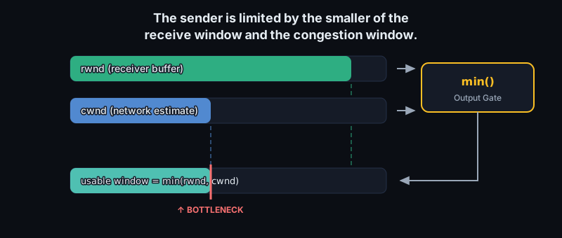
That min matters in low-level work. A receive-window problem is often a host/application problem: slow userspace, small socket buffers, memory pressure, copy overhead, delayed wakeups, or poor receive-side scaling. A congestion-window problem is often a path problem: loss, ECN marks, queue growth, ACK compression, pacing interactions, or competition at a bottleneck. A full RX ring can cause drops that look like network loss to the peer. Large TSO/GSO bursts can dump more bytes into a qdisc or device queue than the pacing model intended. Interrupt moderation can reshape ACK timing.
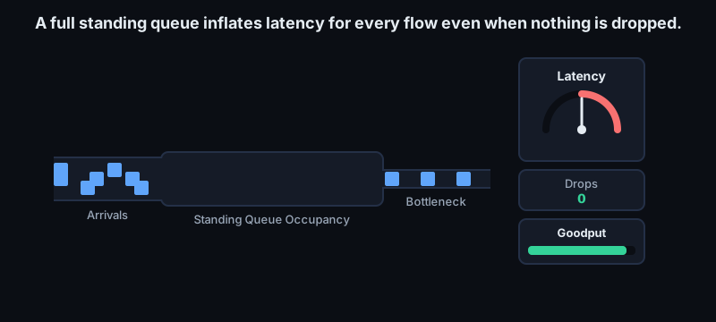
The core goal is not merely “avoid drops.” A network with zero drops can still be congested if bottleneck queues stay full and every flow pays inflated latency. Nor is the goal “maximize one sender.” A shared network must allocate capacity among flows with different RTTs, packet sizes, start times, and implementations. TCP congestion control gives cooperative transports a behavioral contract: probe for capacity, infer overload, and yield enough that other flows can make progress.
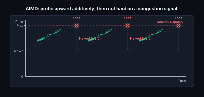
The classic intuition is AIMD: additive increase, multiplicative decrease. Additive increase means probing upward gently. If ACKs keep returning and no congestion signal appears, the sender increases its window by a small amount over time. Multiplicative decrease means backing off hard when congestion is inferred. A loss event is not treated as a request to shave off one packet; it is treated as evidence that the current aggregate offered load exceeded the bottleneck’s sustainable capacity. Cutting the window by a fraction quickly drains pressure from the queue and gives competing flows room.
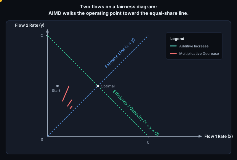
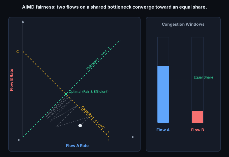
AIMD has a fairness story as well as a stability story. Imagine two long-lived flows sharing one bottleneck. If both increase linearly, their combined load gradually approaches the bottleneck capacity. When congestion occurs, multiplicative decrease pulls both back in proportion to their current rates. Repeating that cycle tends to move cooperative flows toward a fair share while still keeping the link busy. RTT, ACK behavior, queue management, offloads, and the chosen algorithm all affect the exact result, but the shape of the argument is why “probe up gently, back off hard” became the baseline design.
This also explains why congestion control belongs at the endpoints even though congestion happens inside the network. Routers and switches can help by dropping, marking with ECN, scheduling fairly, or running active queue management. Datacenter fabrics can add stronger signals because the operator controls more of the environment. But the sender is where application demand becomes packets. The sender chooses how many bytes are in flight, how bursts are paced, how retransmissions are scheduled, and how quickly a flow recovers after a signal.
The rest of the chapter follows from this feedback-loop view. Slow start asks how a new flow can find capacity without beginning at line rate. Congestion avoidance and AIMD describe the steady-state sawtooth that made classic TCP safe for the shared Internet. Fast retransmit and recovery respond when loss is visible before a timeout. CUBIC changes the probing function for high-bandwidth, high-delay paths. BBR asks whether loss is the wrong primary signal and instead models bottleneck bandwidth and propagation delay. AQM, ECN, DCTCP, and datacenter congestion control tighten the loop where microseconds, shallow buffers, incast, and NIC offloads make old assumptions visible.
The invariant underneath all of them is simple: a sender must not confuse its ability to generate packets with the network’s ability to deliver useful bytes. Congestion control exists because that difference is real, shared, dynamic, and destructive when ignored.
Sources
8.2 Slow start, congestion avoidance, AIMD
Classic TCP congestion control is a sender-side control loop around one variable: the congestion window, cwnd. The receiver window says how much buffer space the peer has advertised; cwnd says how much unacknowledged data the sender believes the network can safely hold. The sender may have at most roughly min(cwnd, rwnd) bytes in flight. The algorithm is about how quickly cwnd should grow, and how sharply it should fall, with only ACK timing and loss as feedback.
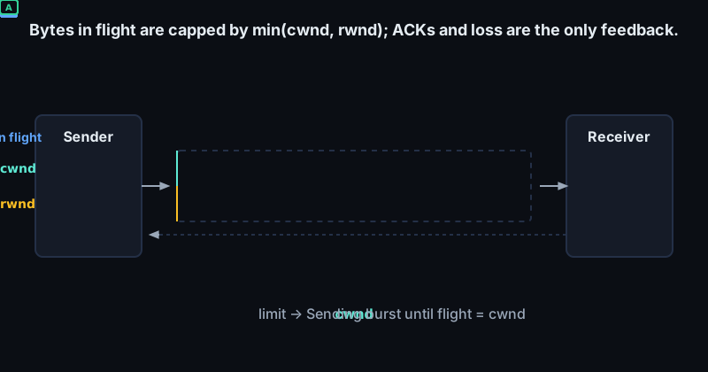
The first problem is startup. A new connection usually has no reliable estimate of the path's bandwidth-delay product. Sending one segment per RTT forever would be safe but wasteful; blasting a full socket buffer into an unknown path can overflow a queue. Slow start is the compromise. Despite the name, it is the aggressive phase: start with an initial window, IW, and increase cwnd by at most one sender maximum segment size, SMSS, for each ACK that cumulatively acknowledges new data. If ACKs arrive for a window's worth of data, the next RTT can send about twice as much as the previous RTT.
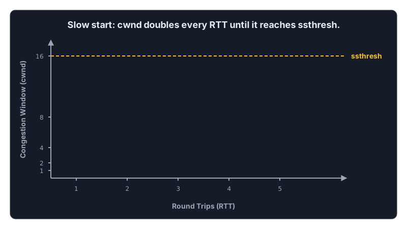
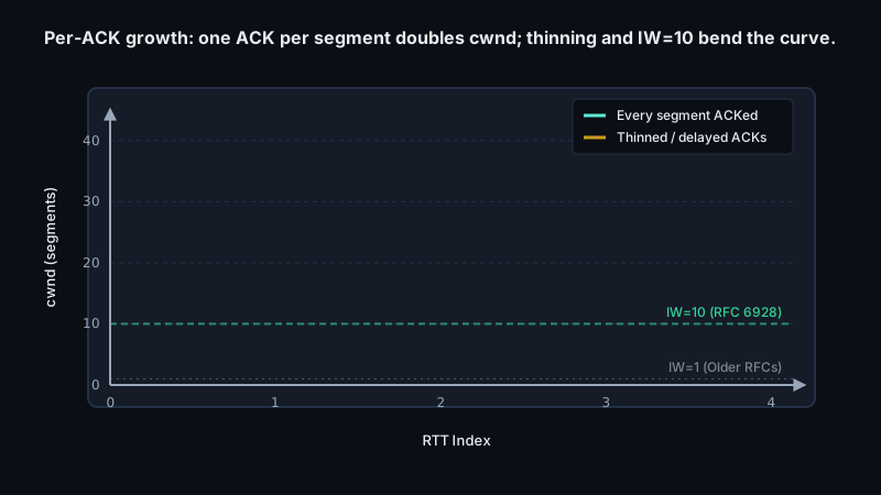
That per-ACK rule matters more than the cartoon. With one ACK per segment, cwnd goes from 1, to 2, to 4, to 8 segments over successive RTTs. With delayed ACKs, ACK thinning, GRO/LRO effects, or application-limited sending, growth is not a perfect power of two. Modern TCP also commonly starts above one segment; RFC 6928 specified an experimental permitted initial window of 10 segments, with fallback guidance. The shape is unchanged: exponential probing, driven by the returned ACK clock, until the sender has evidence that the path is near capacity.
The boundary between the two growth modes is ssthresh, the slow-start threshold. When cwnd < ssthresh, the sender uses slow start. When cwnd > ssthresh, it uses congestion avoidance. At equality, RFC 5681 permits either behavior. After a loss event, ssthresh is set from the current flight size, usually to about half of the outstanding data, subject to a minimum of 2 * SMSS. From then on, ssthresh records a rough memory of where the previous attempt became too aggressive.
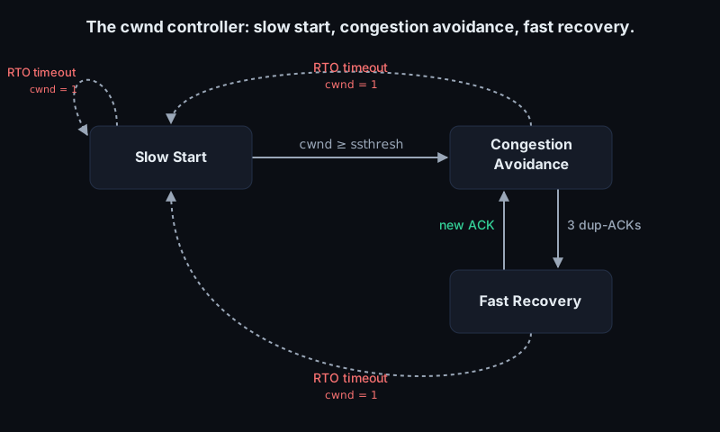
Congestion avoidance is the gentler phase. Instead of doubling each RTT, classic TCP increases cwnd by about one SMSS per RTT. Implementations spread that increase across ACKs: each ACK contributes a small fraction, so a whole window of ACKs adds up to about one segment. This is additive increase. It is slow because the sender has found a plausible operating point and is probing for spare capacity without causing large queue swings.
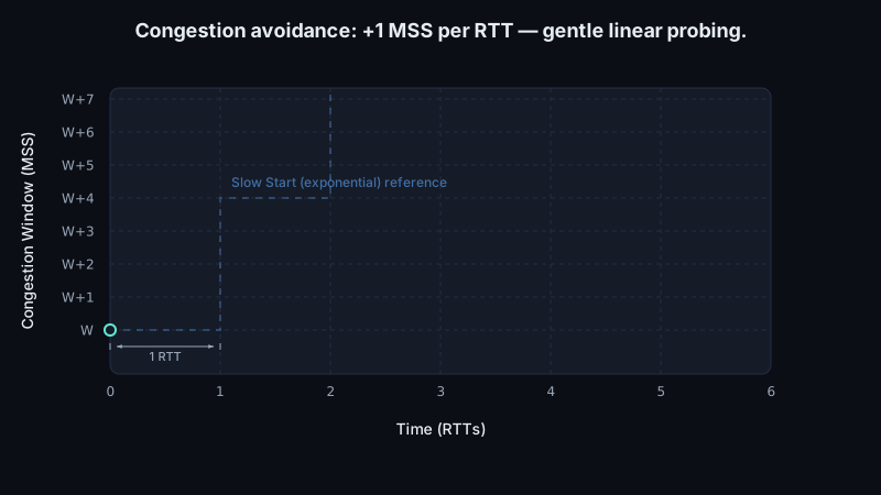
A useful mental model is a single bottleneck queue. If the sender's rate is below the bottleneck's service rate, ACKs come back steadily and cwnd can grow. When aggregate senders exceed the bottleneck, the queue absorbs the burst for a while; eventually either delay grows or packets are dropped. Classic TCP treats packet loss as the congestion signal. On loss, it performs multiplicative decrease: reduce the sending window by a factor, classically one half, and set ssthresh to that reduced value. The full AIMD rule is therefore:
- Additive increase: grow by about one
SMSSper RTT during congestion avoidance. - Multiplicative decrease: on congestion, cut the window sharply, traditionally to about half.
- Slow start: after connection start, timeout recovery, or a low threshold, grow exponentially until
ssthreshis reached.
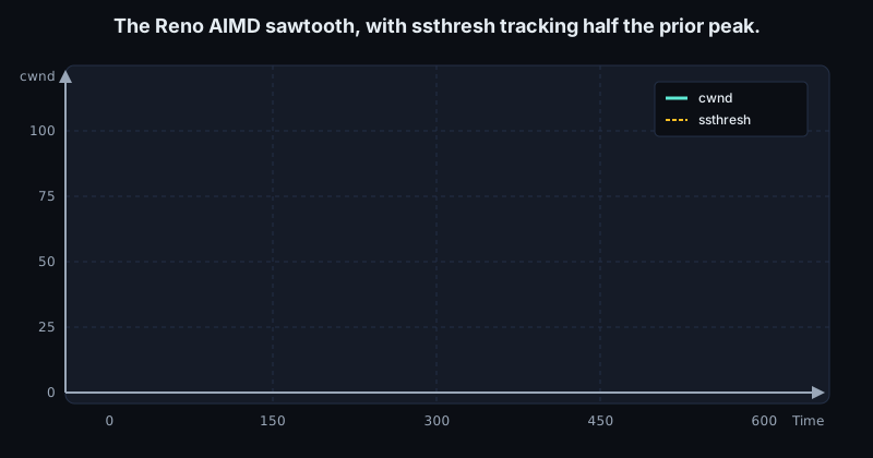
The stability argument is simple but powerful. Additive increase lets competing flows approach capacity without synchronized explosions. Multiplicative decrease drains queues quickly after overshoot. If two Reno-like flows share a bottleneck and see the same losses, the larger flow gives up more absolute bandwidth when both halve their windows, which tends to pull the system toward fairness over repeated cycles. It is not perfect: RTT differences, ACK behavior, offloads, queue policy, and application pacing all matter. But AIMD was the first robust rule that made the public Internet survivable under distributed, uncoordinated senders.
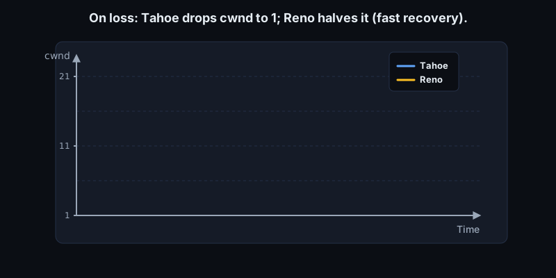
Tahoe, Reno, and NewReno refine what happens after loss. TCP Tahoe introduced the core ideas: slow start, congestion avoidance, and fast retransmit. On detecting loss, Tahoe sets ssthresh to about half the current flight, collapses cwnd to one segment, retransmits, and re-enters slow start. This is reasonable after a retransmission timeout, where the ACK clock may have stopped. But after duplicate ACKs, the receiver is still generating feedback, which implies later packets are reaching the destination.
Reno exploits that distinction with fast recovery. After the usual duplicate-ACK trigger for fast retransmit, Reno retransmits the missing segment, sets ssthresh to about half the flight, and avoids collapsing all the way to one segment. The duplicate ACKs are treated as evidence that packets have left the network and reached the receiver, so the sender can keep data moving. This is the historical shorthand: Tahoe falls back to slow start on this kind of loss; Reno halves and recovers.
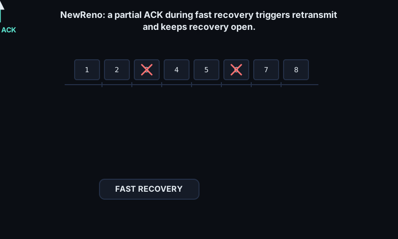
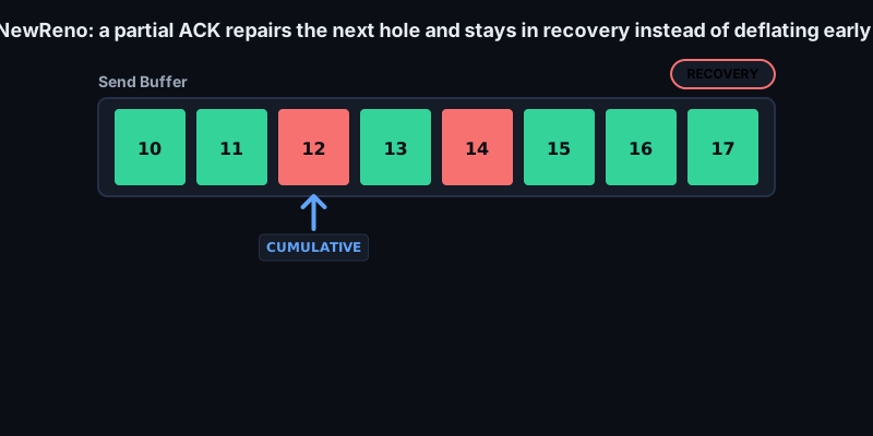
NewReno fixes an important Reno weakness when multiple packets are lost from the same window. A Reno sender can leave fast recovery too early when it receives a partial ACK: an ACK that advances the cumulative acknowledgment point but does not cover all data outstanding when recovery began. NewReno treats a partial ACK during fast recovery as evidence that the next unacknowledged segment is probably lost, retransmits it, and remains in fast recovery until all data from the recovery window has been acknowledged. This is still cumulative-ACK TCP, not SACK-based precision, but it avoids unnecessary timeouts under multiple losses.
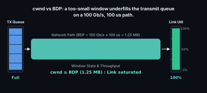
For low-level systems work, cwnd gates real transmit descriptors, DMA mappings, TSO super-packets, pacing decisions, and wakeups. A driver may see a few large TSO buffers while the TCP stack accounts in bytes and segments. A NIC may coalesce completions while the congestion controller is paced by ACKs arriving on another CPU. None of that changes AIMD's contract, but debugging throughput requires looking at bytes in flight, not merely packets handed to the NIC. A 100 Gb/s link with a 100 microsecond RTT has a bandwidth-delay product around 1.25 MB; a small cwnd or a reset to slow start can underfill the transmit queue.
The exponential-then-linear shape is therefore not a historical curiosity. Slow start rapidly discovers an order-of-magnitude capacity estimate. Congestion avoidance continues probing once the sender is close enough that mistakes are expensive. Multiplicative decrease backs off fast enough for shared queues to recover. Tahoe, Reno, and NewReno differ in recovery details, but they share the same control-loop idea: use ACKs to clock growth, use loss to mark overshoot, and converge toward a rate the path can carry.
Sources
8.3 Loss as a signal: fast retransmit and recovery
Loss-based TCP control treats missing bytes as evidence that the path has been overfilled. If a router queue overflows, a packet is dropped; if a packet is dropped, the sender should reduce its sending rate. Fast retransmit and fast recovery let TCP react without waiting for a retransmission timeout. Loss recovery is therefore not just reliability work. It is where the congestion controller decides whether to keep the ACK clock alive at a reduced rate or fall back to slow start.
Duplicate ACKs as a hint: TCP acknowledgments are cumulative. If the receiver has bytes through sequence X, and then receives data above X while byte X+1 is still missing, it cannot advance the ACK number. Instead it sends another ACK for X, often with SACK information if negotiated. From the sender's point of view, repeated ACKs for the same left edge mean: "the receiver is still missing the next byte, but later data has arrived." That is a strong hint that one segment was lost while later segments continued through the network.
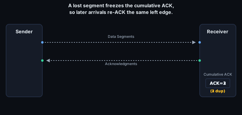
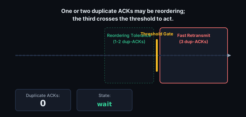
It is only a hint. Later data could have arrived first because the network reordered packets, a NIC path split traffic across queues, a tunnel changed paths, or duplication occurred. Still, the classic rule is pragmatic: after 3 duplicate ACKs arrive without an intervening ACK that advances SND.UNA, the sender assumes the segment at SND.UNA is missing and retransmits it immediately. This is fast retransmit: repair the likely hole before the retransmission timer expires.
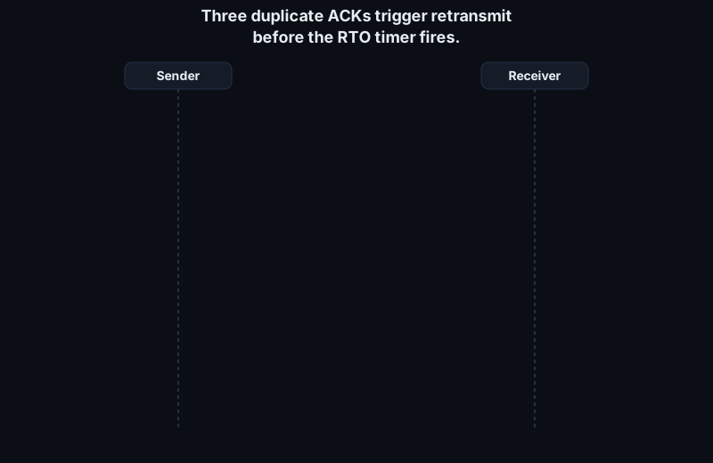
The reason for waiting for three duplicate ACKs instead of one is to avoid punishing harmless reordering. One duplicate ACK is common; two may still be a path artifact; three imply that later segments reached the receiver while the earlier one did not. In a trace, this appears as a run of ACKs with the same ack_seq, often with changing SACK blocks describing bytes received above the gap.
Fast recovery: Fast retransmit repairs the missing segment; fast recovery decides how much the sender may transmit while waiting for the repair ACK. Reno's key observation is that duplicate ACKs prove that some data has left the network. The receiver can only generate a duplicate ACK after receiving a segment above the gap, so each duplicate ACK says one segment is no longer occupying queue or link capacity. The sender should reduce its window because loss suggests congestion, but it need not drain the pipe to zero.
In Reno-style recovery, when the third duplicate ACK arrives, TCP sets ssthresh to roughly half the outstanding data, bounded at max(FlightSize / 2, 2*SMSS). It retransmits the missing segment and sets cwnd = ssthresh + 3*SMSS. The extra 3*SMSS is artificial inflation for the three later segments presumed to have left the network. For each additional duplicate ACK, TCP increments cwnd by SMSS; if cwnd and the receiver window permit, the sender may transmit another segment. This preserves ACK-clocked transmission at a reduced rate.
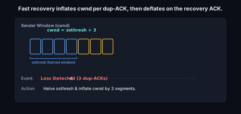
When an ACK finally acknowledges new data, Reno deflates the window by setting cwnd back to ssthresh and resumes congestion avoidance. If the retransmitted segment was the only loss, the cumulative ACK jumps over the repaired gap and covers later data already buffered at the receiver. With multiple losses, basic Reno struggles. The first repair may produce a partial ACK that advances only to the next missing segment. NewReno improves this by staying in recovery on partial ACKs, but without SACK it still learns mostly from the cumulative ACK edge.
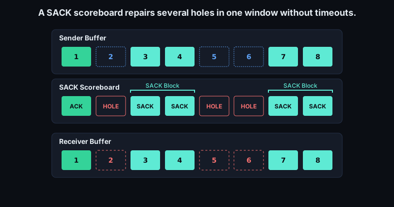
SACK recovery: Selective Acknowledgment changes the sender's visibility. With SACK permitted, the receiver can say, in effect: "I still cumulatively ACK through X, but I also have these byte ranges above X." The sender maintains a scoreboard of sequence ranges that are cumulatively ACKed, selectively ACKed, retransmitted, believed lost, or still possibly in flight. RFC 6675 describes this as an explicit per-connection data structure used to update state from each ACK, estimate pipe, and choose the next segment to send.
That scoreboard makes multiple-loss recovery practical. Suppose a 64-segment flight loses segments 10, 20, and 21, while most later segments arrive. Without SACK, the sender sees duplicate ACKs for segment 10, repairs it, and discovers the next gap only after the cumulative ACK moves. With SACK, the sender can see that bytes beyond 20 and 21 are already present. It can mark the holes lost and retransmit them during the same recovery episode, constrained by the reduced congestion window and pipe estimate. SACK says what likely needs repair; cwnd, ssthresh, and recovery rules limit how aggressively TCP may send.
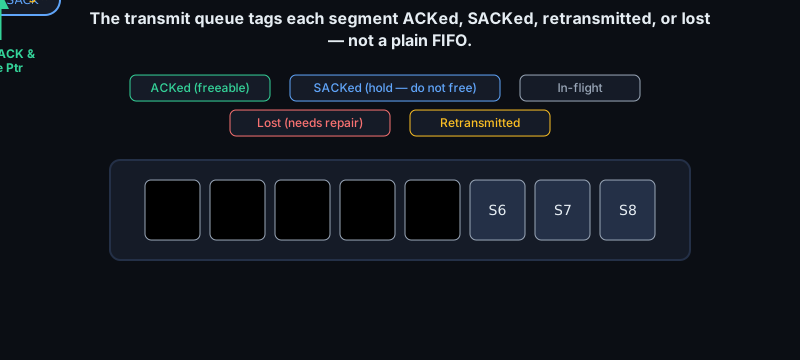
This matters in host networking code because the sender's transmit queue is not a simple FIFO. A TCP stack must keep descriptors for unacknowledged data, tag retransmitted ranges, avoid freeing SACKed bytes until cumulative ACK advances, and decide whether a TSO/GSO aggregate maps cleanly to retransmission units. Driver and NIC offloads can hide packet boundaries unless the stack keeps enough metadata. On receive, GRO/LRO, delayed ACK behavior, and out-of-order queues affect duplicate ACK and SACK timing.
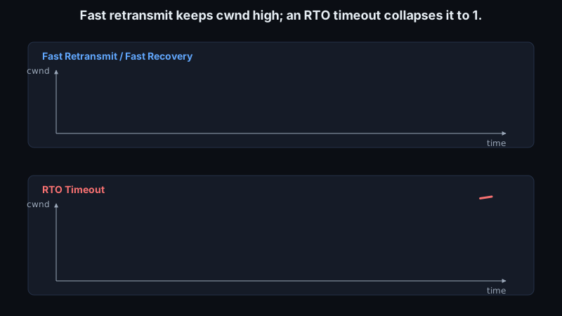
Timeout is the slow path: A retransmission timeout is different from fast retransmit. Fast retransmit fires while ACK feedback is still arriving; the ACK clock is alive, so fast recovery can keep data moving at a reduced rate. An RTO means the sender has not received timely feedback for the oldest outstanding data. TCP therefore takes a much more conservative action: retransmit after the timer, set ssthresh from half the outstanding flight, collapse cwnd to one full-sized segment, and use slow start to rebuild. This is why tail losses and small application-limited transfers are latency-sensitive: there may not be enough later packets to produce three duplicate ACKs.
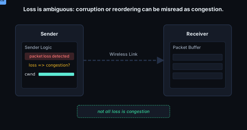
The deeper weakness is that loss is ambiguous. A dropped packet in a full router queue really is congestion evidence. A corrupted wireless frame, reordering on a multipath fabric, a delayed interrupt, or a transient driver queue stall can produce the same duplicate-ACK pattern without bottleneck overflow. Classic loss-based TCP cannot perfectly distinguish these cases. It backs off because doing so is stable for the shared Internet, but the price is needless throughput loss where non-congestion loss or reordering is common. SACK reduces the repair cost. Timestamps and modern time-based loss detection such as RACK use transmission time and SACK feedback to avoid some duplicate-ACK counting failures. Later delay-based and model-based controllers go further by asking whether queues are building before loss occurs.
Sources
8.4 CUBIC and the high-BDP era
Reno's congestion avoidance rule was designed for an Internet where adding roughly one segment per round trip was a reasonable way to search for capacity. After a loss, Reno halves cwnd; while there is no further loss, it grows cwnd linearly by about one SMSS per RTT. The problem is not correctness. The problem is scale.
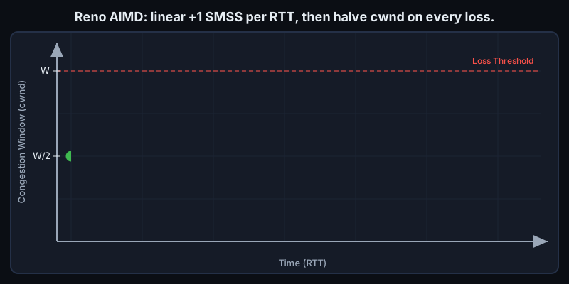
The sender's useful target is the bandwidth-delay product: BDP = bottleneck_bandwidth * RTT. A TCP sender needs roughly that much data in flight to keep the path full. On a 10 Gbit/s path with a 100 ms RTT, the BDP is about 125 MB, or roughly 85,000 full-sized 1460-byte segments. If Reno loses at that point and cuts its window in half, it must climb back by about 42,500 segments. At one segment per RTT, that takes about 4,250 s, or more than an hour.
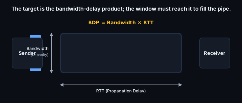
That arithmetic is why high-BDP paths changed the congestion-control problem. A fat, long pipe is filled by maintaining a very large flight size while still backing off when the path says it is overloaded. If the control loop is too timid after every loss, the link spends most of its time below capacity, even when the path has plenty of bandwidth and low corruption.
CUBIC keeps the same broad loss-based contract as Reno: loss, or an ECN congestion indication when enabled, means reduce the sending rate. The important change is how the sender grows cwnd after that reduction. Instead of making the window a linear function of ACK rounds, CUBIC makes the target window a cubic function of real elapsed time since the last congestion event:
W_cubic(t) = C * (t - K)^3 + W_max
Here W_max is the congestion window just before the last reduction, t is time since the congestion-avoidance epoch began, C is the CUBIC scaling constant, and K is chosen so the curve reaches W_max on time. The current Standards Track CUBIC RFC specifies C = 0.4 and recommends beta_cubic = 0.7 for multiplicative decrease.
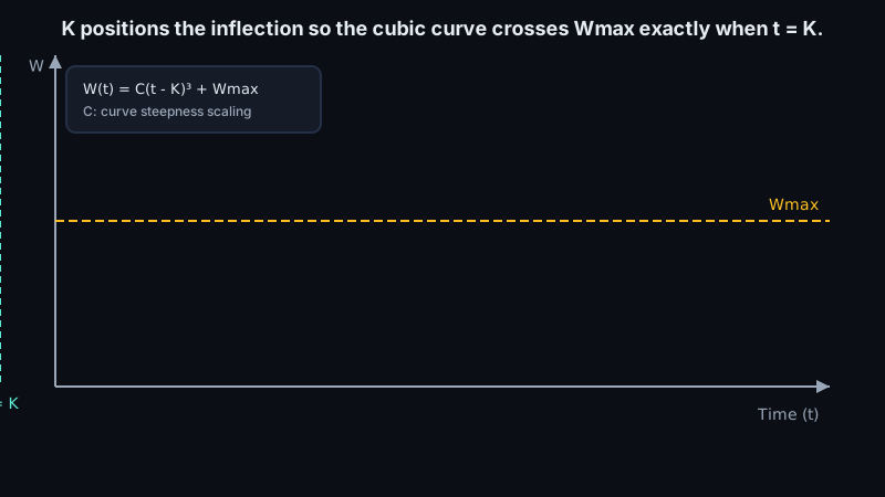
The shape matters more than the formula. After a loss, CUBIC remembers the old high-water mark, W_max, and reduces cwnd less sharply than Reno. Reno's classic multiplicative decrease factor is 0.5; CUBIC's beta of about 0.7 leaves the sender at roughly 70% of the pre-loss flight size. If the old window was near the real BDP, cutting to 50% creates a large empty space in the pipe. Cutting to 70% still relieves pressure, but it does not throw away as much discovered capacity.

From that reduced point, the cubic curve has three intuitive phases.
- Below
W_max, growth is concave. CUBIC increases quickly at first because it is probably reclaiming capacity it already proved the path could carry. - Near
W_max, the curve flattens into a plateau. This is the cautious region: the sender is close to the last observed saturation point, so it avoids charging through it with large bursts. - Above
W_max, growth becomes convex. Now CUBIC is probing for new capacity. If competing flows left, routing changed, or the bottleneck rate increased, the sender can discover a higher operating point.
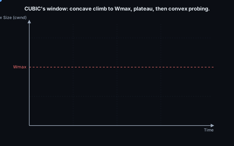
This is a better fit for high-BDP links than Reno's sawtooth. Reno treats every post-loss recovery as a long linear walk. CUBIC treats the last maximum as useful information: return toward that point efficiently, hover around it, then probe beyond it carefully. The plateau is not wasted time. It is a stabilizer around the most likely bottleneck capacity, reducing the chance that many flows overshoot together and synchronize losses.
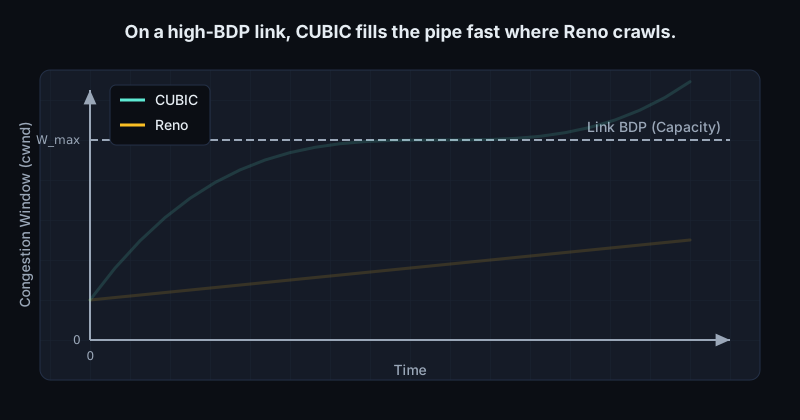
CUBIC is still ACK-clocked in the implementation sense: the sender normally updates cwnd when ACKs arrive, and it still relies on the transport's loss recovery machinery. But the growth target is keyed to wall-clock time rather than to one additive step per RTT. That distinction is central to RTT-independence. In Reno, a flow with a shorter RTT gets more increase opportunities per second. Two flows sharing a bottleneck but seeing different RTTs do not grow at the same rate in real time; the short-RTT flow tends to be more aggressive because its control loop runs more often. CUBIC's cubic target is based on elapsed seconds since the last loss, so outside its Reno-friendly region, flows with different RTTs have much more similar window growth in time.
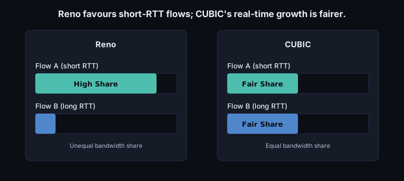
This does not mean every flow gets identical throughput regardless of RTT. Throughput is still approximately cwnd / RTT, and real paths include asynchronous losses, delayed ACKs, offloads, pacing, and queue effects. The narrower claim is that CUBIC avoids making the window-increase law itself proportional to RTT frequency. The RFC describes this as an RTT-fairness improvement over Reno, especially where synchronized loss would otherwise strongly favor shorter RTTs.
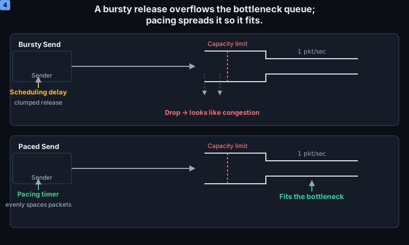
There is a low-level implementation lesson here: congestion control determines how much data the kernel, NIC, and driver are asked to keep moving. A CUBIC flow on a large-BDP path may legitimately need tens or hundreds of megabytes in flight. That interacts with TCP segmentation offload, generic segmentation offload, large receive offload, interrupt moderation, pacing timers, socket buffer sizing, DMA mapping pressure, and ring occupancy. If a send path batches too aggressively and releases a burst after a scheduling delay, CUBIC may see the resulting queue overflow as congestion even though the bottleneck could have carried a paced stream. Modern Linux therefore combines congestion-control choices with pacing, queue disciplines such as fq, accurate byte accounting, and careful timestamping.
CUBIC became the Linux default because it matched the Internet that servers were increasingly operating on: higher access rates, longer paths, larger socket buffers, and enough deployment experience to show that Reno's conservatism was leaving bandwidth unused. Its predecessor, BIC-TCP, had already been selected as a Linux default for high-speed networks, but BIC was more abrupt and less friendly. CUBIC kept the idea of rapidly finding a remembered operating point while replacing binary search behavior with a smoother cubic curve.
The practical mental model is this: the BDP is the window needed to fill the pipe; loss marks a recent upper bound; beta decides how far below that bound to retreat; and the cubic curve decides how to return, hover, and probe. Reno's +1/RTT growth is a good teaching model for AIMD, but it is too slow to be the main workhorse for fast long-distance networks. CUBIC is the engineering compromise that made loss-based TCP scale into the high-BDP era without abandoning the basic feedback loop that made TCP congestion control deployable in the first place.
Sources
8.5 BBR and delay-based control
Loss is a blunt signal. A dropped packet proves that some queue ran out of room, but it does not say when congestion began. By the time loss-based TCP reacts, the bottleneck queue may already be full. Reno and CUBIC can achieve high utilization while also creating large standing queues because they increase inflight data until the network says "enough" by dropping packets or marking ECN.
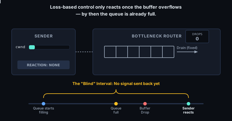
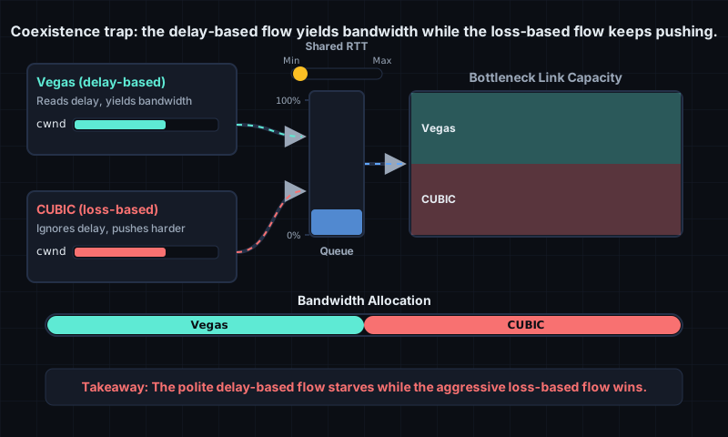
Delay-based control asks a more sensitive question: is the path getting slower before it starts dropping? TCP Vegas is the classic example. Vegas keeps the best observed RTT as a proxy for propagation delay with little queueing. It compares expected throughput, roughly cwnd / baseRTT, with actual throughput, roughly cwnd / currentRTT. If the current RTT rises while cwnd is unchanged, the extra time is usually queueing delay. Vegas interprets the gap as queued data: if the gap is small, increase; if large, back off before loss.
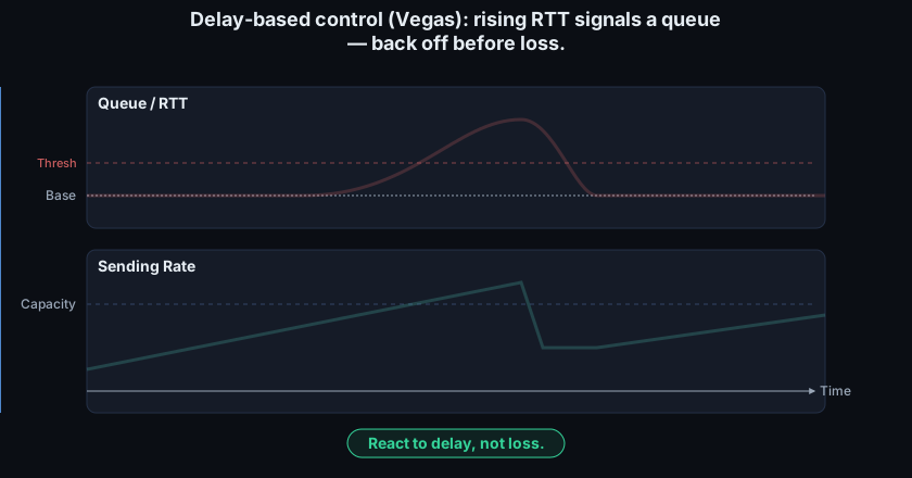
That idea treats a queue as information, not just storage. The problem is coexistence. A Vegas flow that reduces its window when delay rises may share a bottleneck with Reno or CUBIC, which treats the same rising delay as harmless until loss. The loss-based flow keeps pushing; the delay-based flow retreats. In a mixed Internet, delay sensitivity can become a disadvantage.
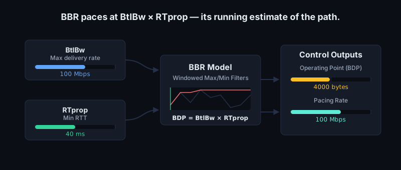
BBR, short for Bottleneck Bandwidth and Round-trip propagation time, takes a different route. It is not purely delay-based like Vegas, and it is not loss-based like Reno/CUBIC. It is model-based. BBR continuously estimates two physical properties:
BtlBw: the bottleneck delivery rate, inferred from recent ACK-clocked delivery-rate samples.RTprop: the minimum round-trip propagation time, inferred from the lowest RTT sample seen over a recent time window.
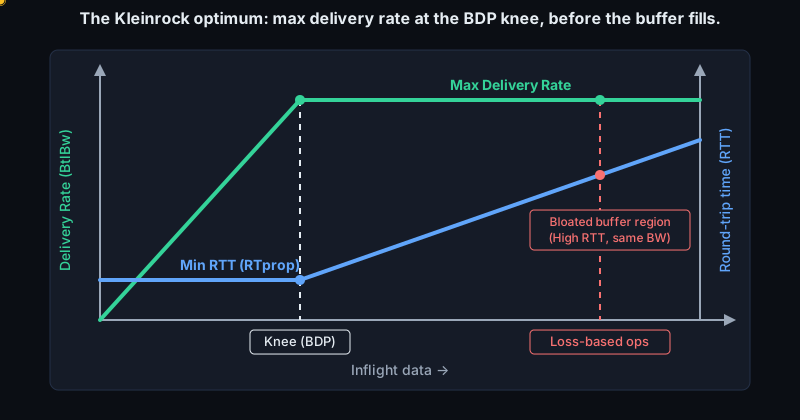
If those estimates are right, the data needed to fill the path but not a persistent queue is their product: BDP = BtlBw * RTprop. Below that inflight level, the pipe is not full. At about one BDP, the bottleneck can run at full rate with little queue. Beyond one BDP, extra packets mostly sit in the bottleneck buffer, increasing RTT without increasing delivery rate. This is the "knee" of the delivery-rate versus inflight curve: throughput is near its maximum, while queueing delay is near its minimum. BBR tries to operate near that Kleinrock optimal operating point.
This framing changes the control problem. A loss-based sender asks, "how much can I put in flight before something drops?" BBR asks, "what rate is the bottleneck delivering, and how much inflight data sustains that rate?" It uses pacing as a first-class control: a pacing rate derived from BtlBw and an inflight cap derived from the estimated BDP. On Linux, this relies on kernel pacing machinery; timestamp quality, ACK processing, segmentation offload, queue disciplines, driver transmit rings, and NIC rate behavior can all affect the packet timing seen on the wire.
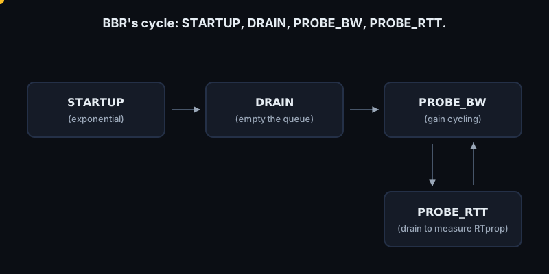
BBR's state machine exists because BtlBw and RTprop cannot be measured perfectly at the same time. To find bandwidth, a sender must sometimes send faster than its current estimate, creating a queue that hides propagation delay. To measure RTprop, it must sometimes reduce inflight data enough for queues to drain.
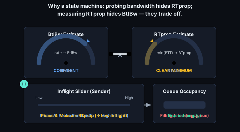
STARTUP is the initial bandwidth search. BBR raises its sending rate rapidly, looking for growth in delivered bandwidth. Once delivery-rate growth stalls, BBR concludes it has likely found the bottleneck rate, but it may have overshot and built a queue.
DRAIN follows. BBR deliberately paces below the estimated bottleneck rate to drain the queue created during STARTUP. The goal is to move from "we found the pipe" to "we are no longer standing on queued packets."
PROBE_BW is the normal long-lived mode. BBR cycles its pacing gain around the estimated bottleneck rate: sometimes above to test for more bandwidth, sometimes below to drain probe-created queue, and often near one times BtlBw to cruise. This is a control loop, not a fixed limiter. Competing traffic arrives and leaves, wireless links shift rates, and virtualized paths can change service rate. BBR keeps sampling ACK-clocked delivery rate and updating the model.
PROBE_RTT refreshes the propagation-delay estimate. Since RTprop is the minimum RTT observed when queues are low, a continuously busy flow may stop seeing clean samples. BBR occasionally reduces inflight data so standing queues can drain and a fresh low RTT can be observed. This costs a short throughput dip, but avoids stale path information.
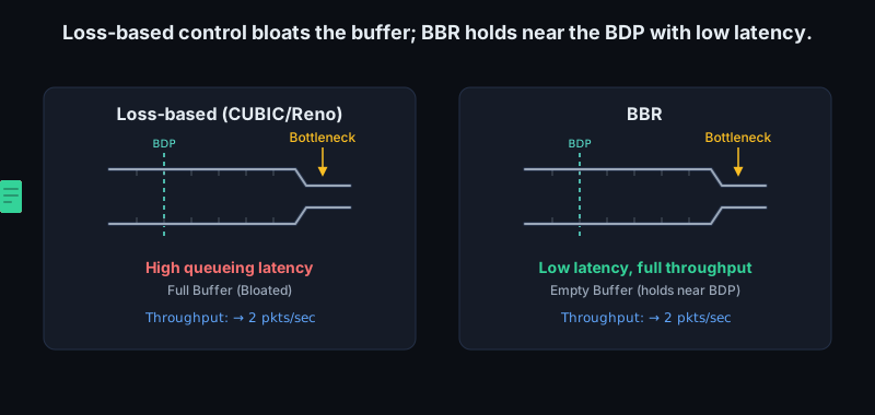
The difference from loss-based control is clearest on a high-BDP path with deep buffers. A CUBIC flow can increase until a large buffer finally overflows, at which point the queue may represent many milliseconds or seconds of excess delay. That hurts RPC tail latency, interactive traffic, and incast recovery long before bulk throughput looks bad. BBR attempts to stop near the BDP instead of the buffer limit, so it can do well where random loss is not congestion, buffers are shallow, or bufferbloat would dominate latency.
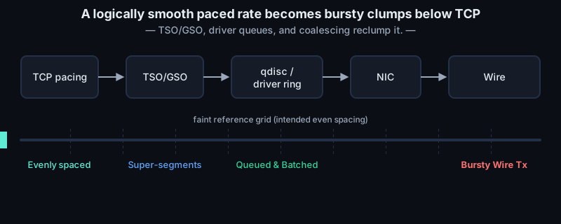
But BBR is not magic fairness dust. Its behavior depends on measurement, pacing, and coexistence. Early BBR versions could be unfair to CUBIC or to other BBR flows in some RTT and buffer regimes. ACK aggregation, policers, token-bucket shapers, and delayed ACKs can distort delivery-rate samples. If pacing is implemented poorly, bursts can reappear below TCP: large TSO/GSO segments, deep driver queues, interrupt moderation, or NIC offloads can turn a smooth logical rate into clumps on the wire.
These details matter in datacenters. BBR's model is attractive because it tries to minimize standing queues while preserving throughput, but fabrics often use additional signals such as ECN and algorithms such as DCTCP because microsecond-scale queues, shallow switch buffers, and many-to-one incast require fast feedback. A host TCP stack, NIC driver, and switch AQM policy are one control system. If the host holds packets in a qdisc or driver ring after TCP thinks they were paced, TCP's model includes local buffering. If ACK timestamps are noisy because of batching, GRO/LRO, or interrupt coalescing, the delivery-rate estimator can be biased.
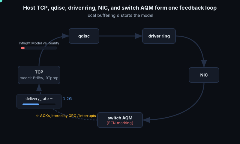
The deeper lesson is that congestion control is not only an algorithm in tcp_cong.c. It is a distributed feedback loop implemented with clocks, queues, DMA rings, ACK generation, offloads, switch buffers, and send patterns. Vegas showed that rising RTT contains early congestion information. BBR showed that a sender can model the pipe: estimate the bottleneck rate, estimate propagation delay, pace near BtlBw, and keep inflight data near BtlBw * RTprop. The debates are about measurement accuracy, probing aggressiveness, and fairness when control laws share one bottleneck.
Sources
8.6 Fairness, AQM, and datacenter congestion
Fairness under additive increase. AIMD has a useful geometric property when competing flows run the same algorithm over the same bottleneck and see roughly the same RTT. Imagine two long-lived Reno-like flows sharing one link. Each RTT, both increase cwnd by about one MSS. The offered load walks upward until the queue overflows or the AQM marks congestion. Then both flows multiplicatively reduce. If one flow has a larger window, the same cut removes more bytes from it than from the smaller flow. Repeating this cycle pulls the pair toward equal rates while keeping the bottleneck busy.
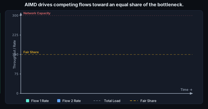
That fairness is conditional. A flow with a shorter RTT runs the additive-increase loop more often per second, so classic TCP is biased toward short-RTT paths. Fairness also breaks when algorithms interpret the same signal differently. Reno halves on loss; CUBIC usually reduces to 0.7 * W_max; BBR may not treat isolated loss as proof that the bottleneck rate fell; DCTCP reduces in proportion to ECN marking fraction. Mixing them in one queue can be unfair. For low-level engineers, a packet capture that says "TCP" is not enough: congestion module, RTT, ECN negotiation, pacing, offload behavior, and queue discipline all shape the actual rate.

Queue management. The simplest router or switch policy is drop-tail: enqueue until the buffer is full, then drop arriving packets. This absorbs bursts, but it gives endpoints feedback only after the queue has become a latency machine. Large buffers can hide congestion for many RTTs, producing bufferbloat: high standing delay, jitter, and synchronized losses.
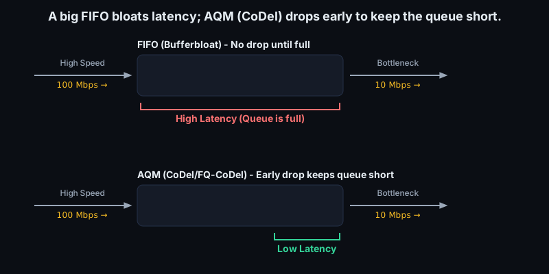
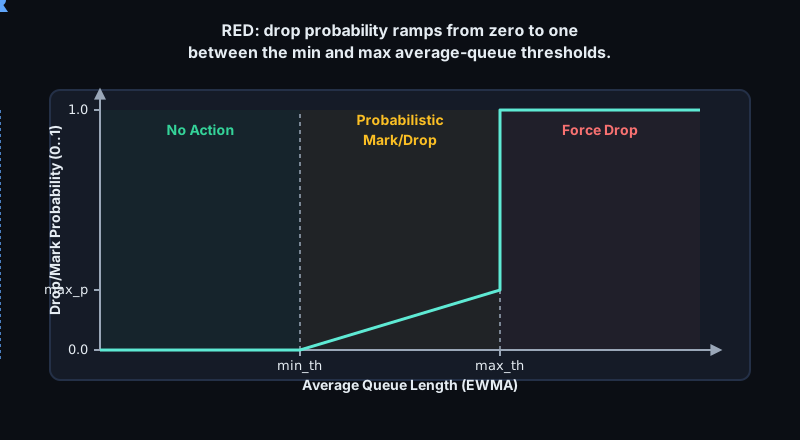
Active Queue Management moves the signal earlier. RED, the classic Random Early Detection algorithm, keeps an exponentially weighted average queue length. Below a minimum threshold it does nothing. Above a maximum threshold it drops or marks every arriving packet. Between the thresholds it drops or marks with increasing probability. The idea is to avoid hard overflow and synchronized loss, while making a flow's chance of receiving a signal roughly proportional to its queue share. RED separated "the buffer is out of memory" from "tell senders to slow down," but its thresholds were hard to tune.
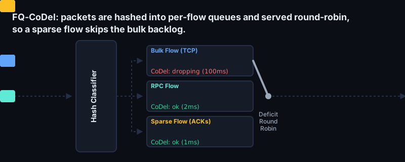
Modern AQM controls delay more directly. CoDel measures how long packets sit in the queue and reacts when the minimum sojourn time over an interval remains above a target; the minimum filters out harmless short bursts. PIE also targets average queueing delay, adjusting drop or mark probability with a lightweight control loop. FQ-CoDel adds flow queueing: packets are classified into per-flow queues, served with a deficit round-robin style scheduler, and CoDel runs inside those queues. This gives sparse flows, RPCs, ACKs, and interactive traffic isolation from bulk transfer head-of-line blocking.
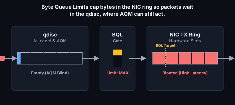
On Linux hosts, this reaches into the driver boundary. Byte Queue Limits, transmit ring sizing, sch_fq, fq_codel, pacing, TSO/GSO segmentation, and NIC completion timing all affect where packets wait. If too much data sits in a device ring, the kernel qdisc may have no opportunity to pace, drop, or mark intelligently.
ECN as lossless signalling. Explicit Congestion Notification gives AQM a cleaner signal path. With ECN negotiated, the sender marks IP packets as ECN-capable using ECT(0) or ECT(1). A congested router or switch can set the CE codepoint instead of dropping the packet. The TCP receiver echoes the signal with ECE; the sender reduces its congestion window and acknowledges that response with CWR. The payload was delivered, so congestion was signalled without retransmission.
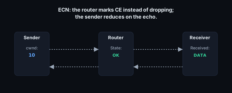
ECN does not eliminate congestion control. It changes the evidence. A CE mark means "this packet crossed a congested queue"; the sender must still reduce load. It also depends on host stack, tunnels, NIC offload path, switch AQM profile, and middleboxes preserving the bits. In datacenters, marking thresholds and endpoint behavior can be engineered together.
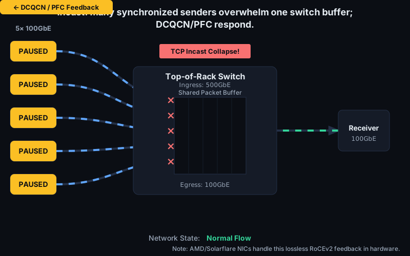
Datacenter congestion. Datacenter networks have small RTTs, high link rates, shallow switch buffers relative to bandwidth, and bursty workloads: RPC fan-in, storage reads, distributed training collectives, and cache misses. A few dozen senders can synchronize on one receiver and overflow the top-of-rack switch queue before classic TCP infers anything from loss. This is incast. The issue is not average utilization; it is many flows becoming runnable at once and converging on one egress port or host.
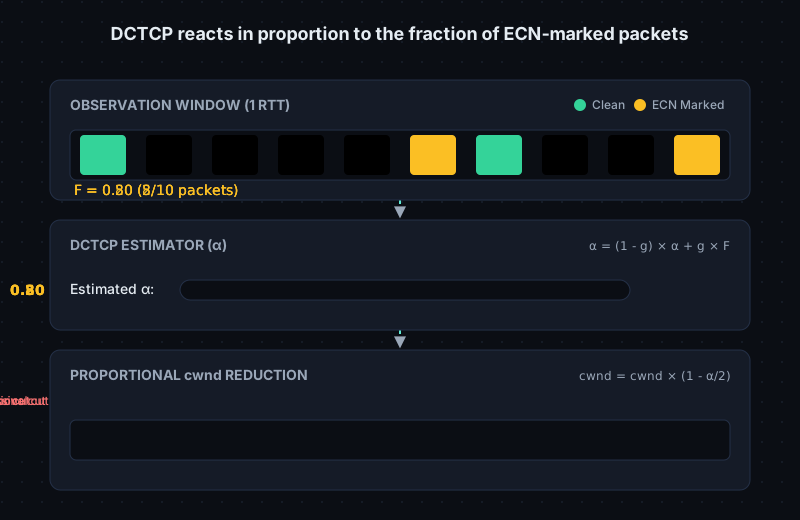
DCTCP was designed for that environment. Switches mark packets with CE once a shallow queue threshold is crossed. The receiver reports ECN marks, and the sender estimates the fraction of marked packets, often represented as alpha. Instead of halving cwnd on one congestion indication, DCTCP reduces proportionally: heavy marking causes a large reduction, light marking causes a small one. The control loop can keep queues short while maintaining high throughput, but it assumes consistent ECN support and carefully chosen thresholds. RFC 8257 warns that DCTCP and conventional TCP should usually be segregated because they do not share capacity like identical AIMD flows.
RDMA over Converged Ethernet raises the stakes. RoCE is attractive for HPC and AI fabrics because the NIC can move data directly between application buffers with low CPU overhead, but RoCEv2 runs over UDP/IP and expects a very low-loss Ethernet fabric. Packet loss can be far more expensive than with ordinary TCP because recovery may involve NIC transport state or upper-layer stalls. Operators therefore deploy Priority Flow Control, PFC, from IEEE 802.1Qbb. PFC pauses a traffic class on a link before buffers overflow.
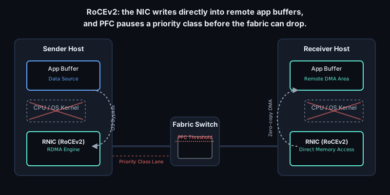
PFC is blunt. It is link-local, not end-to-end; it pauses a priority class, not just the guilty flow; and if misconfigured it can spread congestion backward or create head-of-line blocking. DCQCN, Data Center Quantized Congestion Notification, combines ECN marking in switches with end-host/NIC rate control for RoCEv2. The switch marks congestion, the receiver returns congestion notification, and the sender reduces and later increases its injection rate. PFC remains as a safety net, while ECN/DCQCN should do the normal control work early enough that pause frames are rare.
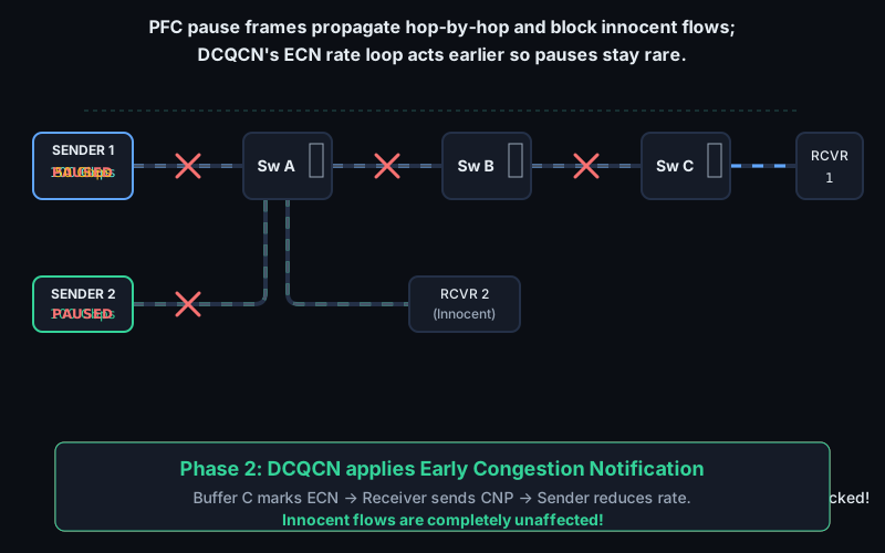
This is directly in the wheelhouse of Solarflare-style NIC and driver work. The questions are where ECN marks are generated and reflected, how completion queues behave when PFC pauses a class, how hardware rate limiting interacts with software pacing, and what telemetry exposes microbursts before they become drops or stalled GPU collectives. Datacenter congestion control is not just a TCP algorithm in the kernel. It is a feedback system spanning application burst shape, kernel queues, NIC rings, switch buffers, ECN thresholds, pause headroom, and firmware rate control.
Sources